How earthquake science supports decision-making in the ancient continent
Mark Quigley1,2, Adam Pascale2, Wayne Peck2, Dee Ninis2, Elodie Borleis2, Russell Cuthbertson2
(1) School of Geography, Earth & Atmospheric Sciences, The University of Melbourne VIC 3010, Australia (2) Seismology Research Centre, Richmond VIC 3121, Australia
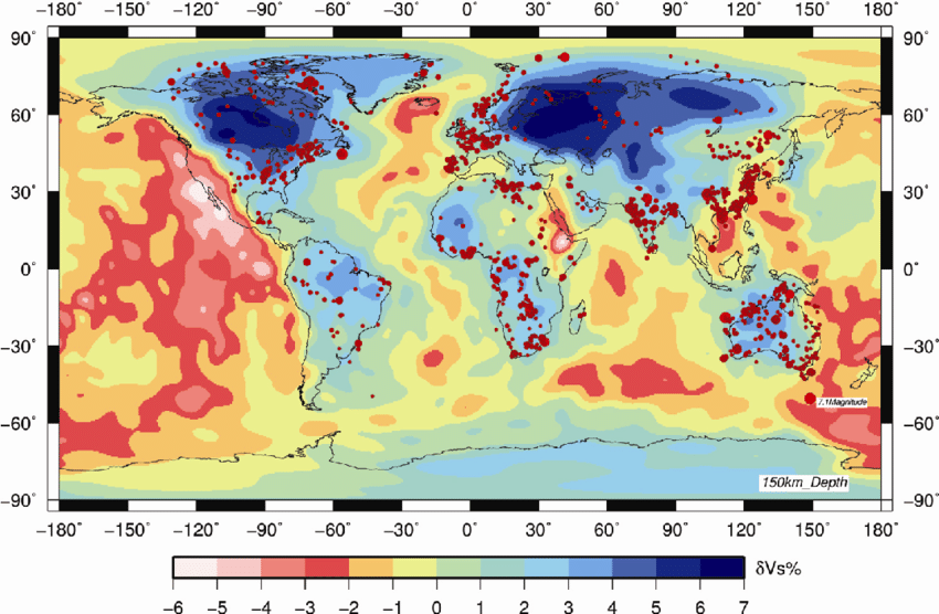
Approximately 80% of the Australian continent is comprised of very old (> 0.54 to 4.4 Billion years) continental crust within thick (>180 to 280 km) and strong lithosphere (Figure 1). When compared with analogous geological settings, commonly referred to as Stable Continental Regions (SCRs), Australia is amongst the most seismically active (Figure 1).
There is a widely held perception that potentially destructive earthquakes in Australia are rare. However, Australia experiences earthquakes analogous to the catastrophic 2011 moment magnitude (Mw) 6.2 Christchurch, New Zealand earthquake (185 fatalities) and its damaging Mw ≥ 6.0 aftershocks (collectively totalling > $30 billion AUD damage) every 6 to 20 years on average. Since 1960, the Australian continent has hosted ten Mw ≥ 6.0 earthquakes (7 on land, 3 offshore).
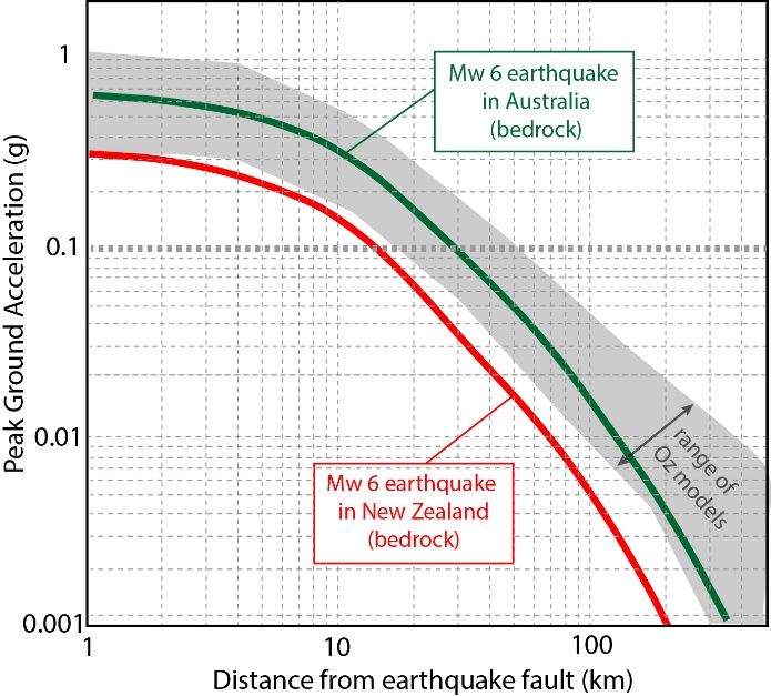
The strong Australian crust enables potentially damaging seismic waves to travel further (relative to the earthquake fault rupture source) compared to many plate boundary regions like New Zealand. This effect is typically estimated using ground motion models (GMMs) (Figure 2) that plot a measure of ground shaking intensity, like peak ground acceleration (PGA) against distances from earthquake epicentres or defined fault ruptures. In the example below, it is suggested that PGAs of 0.1g may be expected at distances of ca. 30 km from an earthquake source fault in Australia compared to roughly half that distance (ca. 15 km) from an earthquake source fault in New Zealand. In many settings, there is uncertainty in the selecting the most appropriate GMM to represent the expected shaking conditions in future earthquakes. Scientists may therefore use a variety of GMMs and analytic techniques such as weighted logic trees to represent the range and uncertainty of model outputs in seismic hazard modelling.
When coupled with dense populations in areas of lower seismic building code standards (relative to more seismically active countries) and vulnerable infrastructure, the damage and loss of life in an Australian earthquake beneath one of our urban centres could substantially exceed that expected for a similar magnitude earthquake in many plate boundary regions in socio-economically comparable countries.
A conceptual model of Australia seismic hazard
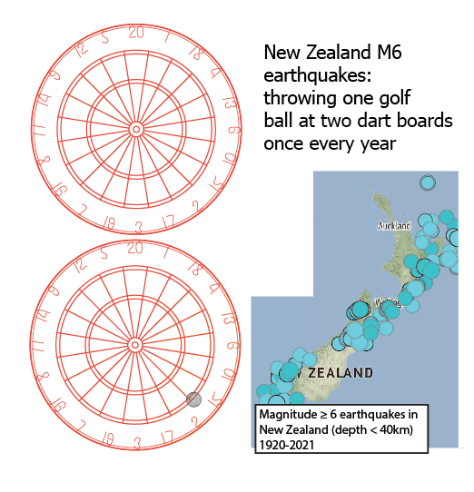
To conceptualize seismic hazard in Australia relative to our neighbours on the Shaky Isles, we offer the following analogy (Figure 3). Picture, on one hand, lobbing a golf ball (a scaled-down representation of the area over which potentially damaging seismic waves might be felt for a shallow, Mw 6.0 crustal earthquake) at an area equivalent to two dart boards (a scaled-down approximation of the terrestrial land area of New Zealand) once every year. Depending on one’s aim and intention, golf ball impacts may tend to cluster in certain areas of one board or another (i.e., more tectonically and seismologically active areas of the plate boundary). And occasionally, golf ball impacts may strike more peripheral areas of the boards, analogous to less frequent, strong earthquakes in the more slowly deforming peripheries of the plate boundary. The latter instance is a reasonable portrayal of the 2011 Christchurch earthquake.
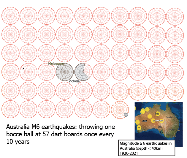
Now consider a much larger target area (57 dart boards representing a scaled-down Australia) and a slightly larger ball (e.g., a bocce ball, representing the potentially larger area over which strong ground shaking might be felt in a Mw 6.0 earthquake) (Figure 4). The bocce ball is being lobbed less frequently (e.g., once every 10 years to represent a lower rate of earthquakes) and with poorer aim (i.e., more randomly distributed earthquakes in a slowly deforming continental region). The relative area of a major metropolitan area like Melbourne could be represented by the inner bullseye on one dartboard and the state of Victoria could be represented by 1 ¾ dartboards. Earthquakes like the 21 May 2016 Mw 6.0 Petermann earthquake in central Australia could be represented by a single bocce ball impact in an area of very low population density and minimal infrastructure. Over the average lifetime of an Australian (ca. 80 years), approximately 8 of these major impacts would be expected to occur somewhere, on a fractionally small proportion of a dart board. Approximately 3 more impacts might miss the dart boards but cause strong shaking on proximate parts of the boards. Inevitably, with enough tosses of the bocce, more vulnerable targets will be impacted. And because of the Gutenberg-Richter relationship for earthquakes, for every bocce ball thrown, many smaller balls (smaller magnitude earthquakes) are also thrown. An example of the impact of one of these smaller balls can be represented by the 28th December 1989 Mw 5.4 Newcastle earthquake (13 fatalities, 50,000 damaged buildings, $3.2 billion AUD damage).
At any specified location on a dart board, the seismic hazard may be represented by the anticipated frequency of golf ball or bocce ball impacts over a given increment of time. The dimensions of these balls represent the approximate (scaled) area over which potentially damaging peak ground accelerations of 10% of gravity (i.e., 0.1 g PGA) could be expected to occur in a Mw 6.0 crustal earthquake. The frequency at which the balls are tossed represents the average Mw 6.0 earthquake frequency in these countries. Areas with increased concentrations of prior impacts are expected to have increased probability for future impacts (we call this earthquake spatial and temporal clustering) although an impact can occur anywhere at any time. In the New Zealand case, the hazard is higher on every part of the two dart boards because balls are being thrown more frequently at a substantially smaller area. In the Australian case, the hazard is substantially lower, even with the larger radius ball. The exposure of a critically important asset to seismic hazard, like a large dam-based reservoir that supplies drinking water to millions of citizens, or a power plant that supplies our electricity, or a planned nuclear waste storage facility, is substantially lower in Australia. However, the risk of an impact is fundamentally important to characterise because socio-economic and life-safety risks from failure (relating to the hazard, exposure, and vulnerability of the asset to seismic shaking and ground rupture) can be lowered with enhanced knowledge of future earthquake scenarios and a better understanding of uncertainty.
How earthquake science empowers decision-making
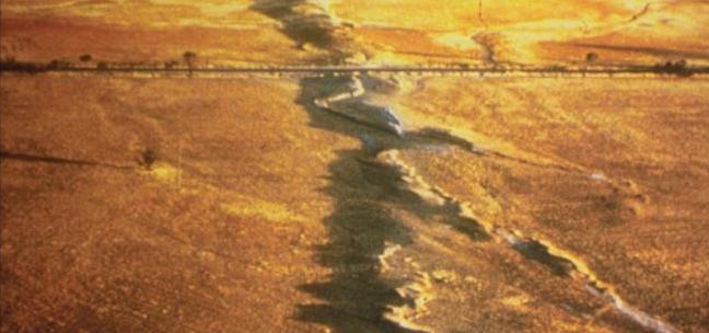
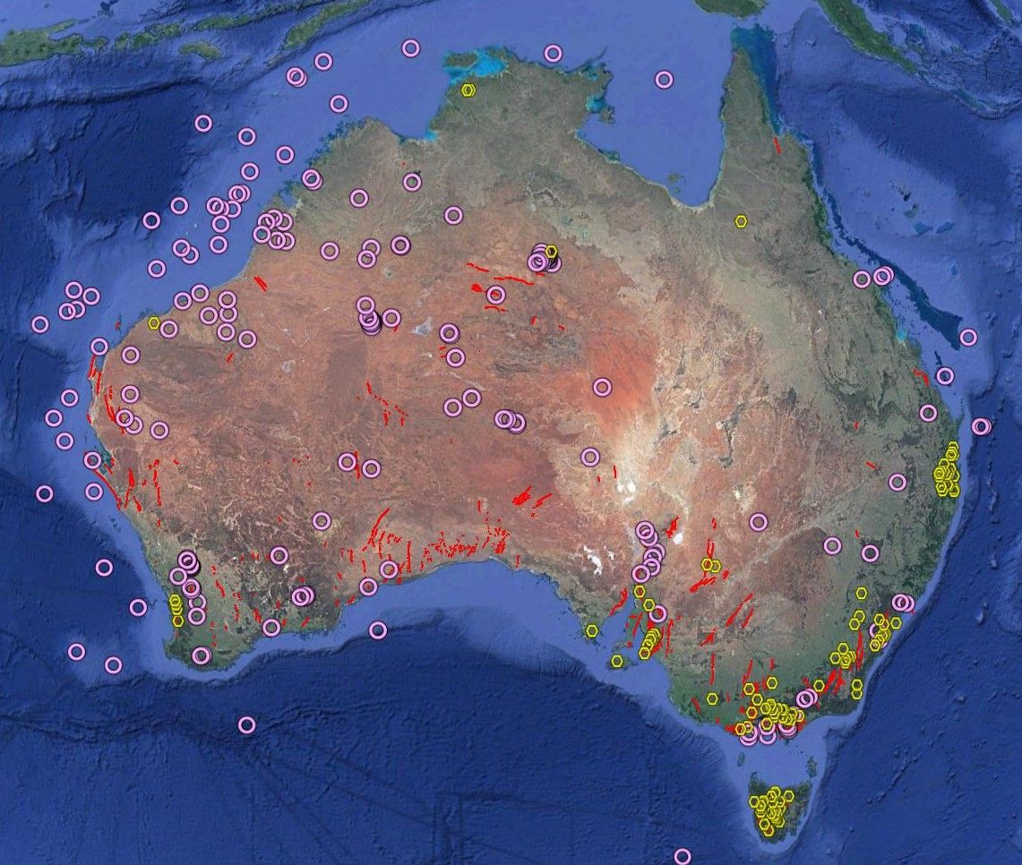
Many of Australia’s most important assets are located in areas of neotectonic faulting and historical seismicity. For example, approximately 80% of Australia’s large dams (Figure 5; yellow hexagons) are located within 100 km of neotectonic faults (Figure 5; black lines) and / or areas of significant seismicity (Figure 5; pink circles – locations of Mw ≥ 5 earthquakes since 1960). There is a good reason for the close relationship between Australia’s neotectonic faults and dams. Faults create topography by breaking and uplifting the rocks relative to surrounding areas. Rivers incise into this uplifted rock to create steeper and deeper valley systems. The best locations for many dams are therefore near the locations of fault-induced topographic changes, where river systems in the uplifted rock can be dammed to create voluminous reservoirs in the valley systems upstream of the dam.
Many of Australia’s largest cities are also located in areas of neotectonic faulting, more frequent earthquakes, and consequently higher seismic hazard. As such, earthquakes pose a high consequence – low likelihood risk that is widespread across the continent. The seismic safety of much of Australia’s important infrastructure is partially dependent upon evaluating seismic hazards and the risks they pose.
It is a public responsibility of owners, operators, regulators, and governments (i.e., ‘decision-makers’) to ensure the safety of critical infrastructure, such as dams, against failure of all types, including that induced by earthquake shaking and ground surface ruptures.
One aspect of this responsibility is to ensure that seismic hazard in the area of the dam is sufficiently characterised and monitored. Our role as earthquake experts is to provide answers to questions such as:
- Are neotectonic, seismically active, and /or potentially active faults (e.g., bedrock faults or other optimally oriented anisotropies such as foliations) present beneath, or in close proximity to, proposed or existing infrastructure?
- What are the expected future behaviours and characteristics of earthquakes in the region of interest (e.g., where, how frequent, how large, how intense the shaking, how much ground displacement might be at a specified location)?
- How exposed is the proposed or existing infrastructure to seismic hazards (shaking, fault rupture, mass movements, liquefaction, etc)?
To answer these questions, we map and study faults in the Earth’s crust using (i) laser scans and photogrammetric models of the earth surface acquired from drones, larger aircraft, and satellites, (ii) geophysical imaging techniques, and bore-hole data that allow us to map faults at depths of several metres to several kilometres, (iii) monitoring and analysis of seismicity to identify active movements on crustal faults to depths of 10s of kms, and (iv) forensic (i.e., trenching) excavations across faults that allow us to determine the timing, displacements, rupture lengths, and frequency of major earthquakes from careful geo-detective work. We record and analyse earthquakes on networks of seismometers to determine their rates and distributions, including any changes related to natural or anthropogenic processes (e.g., ground water withdrawal, reservoir filling).
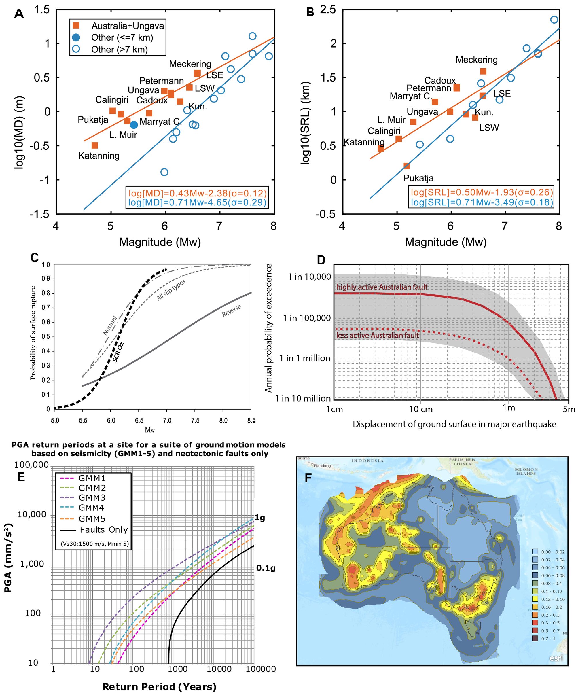
We use things like scaling relationships to estimate the Mw of pre-instrumental earthquakes where our detective work has uncovered past displacements and fault rupture lengths (Figure 6A,B).
For assessing ground surface rupture hazard, we use empirically developed curves that show the probability of earthquakes with specific Mw and rupture kinematics (e.g., normal, reverse faulting) rupturing the ground surface (Figure6C).
We combine these with different types of earthquake data (e.g., how fast the faults have moved over geodetic or geological time-scales) to undertake Probabilistic Fault Displacement Hazard Analyses (PFDHA). PFDHA provides decision-makers with an estimate of the return period of different amounts of ground surface rupture displacements at a specified location (Figure 6D). PFDHA results suggest earthquakes on typical Australian neotectonic faults could be expected to create a 1-meter-high ground surface rupture (surface scarp) once every ca. 80,000 to > 1 million years on average, depending largely on the fault slip rates. An important caveat here is that many Australian faults exhibit spatial and temporal clustering behaviours (e.g. Clark et al., 2012), meaning that the hazard could also be significantly higher, for faults in a more active phase relative to long-term ‘average’ slip rates, or lower, for faults in a more dormant phase. Geological investigations are essential to estimate fault geometries and slip rates, and to improve the accuracy of PFDHA.
Instrumental earthquake records are derived from analyses of seismic waves recorded by seismometers. Statistical analyses of earthquake magnitude-frequency relationships are combined with neotectonic fault data and GMMs (Figure 2) to produce hazard curves, that provide information such as the average return period of ground shaking intensities at specific sites of interest (Figure 6E). Seismic hazard may also be presented as maps that show probabilities of expected intensities of shaking for a specific time period (e.g., Figure 6F, which shows 2% probability of exceedance of a specific ground shaking intensity within a 50-year time period across the Australian continent).
The geological and seismological evidence we provide to decision-makers is only one piece of a rather complicated and technical puzzle that includes modelling and analysis of the expected engineering behaviour of the infrastructure under different conditions of seismic loading (and many other hazards such as large floods), and considerations of how best to sustain, upgrade, (re)build, (re)locate, and / or (re)design infrastructure to minimize risks of failure.
Decision-makers have typically sought to mitigate risks to some level of societal acceptance, commonly referred to as ALARP (as low as reasonably practicable). However, as increasingly evidenced in Australian legislation and case law, decision-makers may now be more commonly required to demonstrate safety due diligence in a way that can withstand post-event judicial scrutiny. The test has transitioned from risk acceptability, to evaluating whether risk mitigation was undertaken to the point that no further reasonably practicable precautions (so far as is reasonably practicable) are available to decision-makers, and that what results is not prohibitively dangerous.
Earthquake science supports decision-making by empowering decision-makers with defensible analyses of seismic hazard, risk, and uncertainty in ways that demonstrate due diligence in the process of knowledge acquisition. Ultimately, earthquake science may not be the definitive factor in risk assessments, site selection and engineering design. Other hazards (e.g., floods, fires, contaminated soils, landslides) may contribute more risk, and socioeconomic and political factors (e.g., cost benefit analyses, societal priorities) may strongly influence the trajectory of decision-making. There are numerous examples, however, of how the incorporation of earthquake science into decision-making has reduced loss and increased community safety, from the grand tale of the Trans-Alaska Oil Pipeline, to the importance of building codes in saving lives and reducing loss. Amidst Australia’s booming expenditures on critical infrastructure, it is imperative that earthquake risks remain a conversation point, and that decisions are informed by best-practise seismic hazard analyses.
References
Allen, T. I., Griffin, J. D., Leonard, M., Clark, D. J., Ghasemi, H. (2020). The 2018 national seismic hazard assessment of Australia: Quantifying hazard changes and model uncertainties. Earthquake Spectra, 36, 5-43.
Clark, D., McPherson, A., & Van Dissen, R. (2012). Long-term behaviour of Australian stable continental region (SCR) faults. Tectonophysics, 566, 1-30.
Horspool, N.A., Chadwick, M.., Ristau, J., Salichon, J., Gerstenberger, M.C. (2015) ShakeMapNZ: Informing post-event decision making, Paper Number O-40, New Zealand Society for Earthquake Engineering,https://www.nzsee.org.nz/db/2015/Papers/O-40_Horspool.pdf
Schulte, S. M. and Mooney, W. D., (2005) An updated global earthquake catalogue for stable continental regions: reassessing the correlation with ancient rifts. Geophys. J. Int., 2005, 161(3), 707–721.
Singh, S., Agrawal, S. Ghosh, A. (2017) Understanding deep earth dynamics: a numerical modelling approach, Current Science, 112, 7, 10 April 2017
Yang, H., Quigley, M., King, T. (2021). Surface slip distributions and geometric complexity of intraplate reverse-faulting earthquakes. GSA Bulletin, https://doi.org/10.1130/B35809.1.
Editor: Louis Moresi