How is 'social distancing' maintained between strike-slip faults?
We have all become highly sensitive to 'social distancing' since the COVID-19 pandemic swept across the Earth. The act of social distancing (more correctly called 'physical distancing') is to keep a safe space between yourself and other people who are not from your household. The safe distance is suggested to be at least 6 feet (about 2 arms’ length). Even in normal times, without any epidemics, people naturally space themselves apart from others that they don't know.
The criteria of a safe distance may vary for other reasons. For example, an emperor would like to have a safe distance at least 10 steps from people except intimate servants and bodyguards. That means the distance may inform us about the internal interactions within a system — something we can observe from a distance.
Fault interactions in nature can be treated as a hierarchical system. Sub-parallel arrays of evenly-spaced faults with comparable length are common to see in different strike-slip shear zones. Active fault spacing in the East Californian Shear Zone (ECSZ) is tens of kilometers while in the Tibetan Plateau it is hundreds of kilometers (see Figure 1).
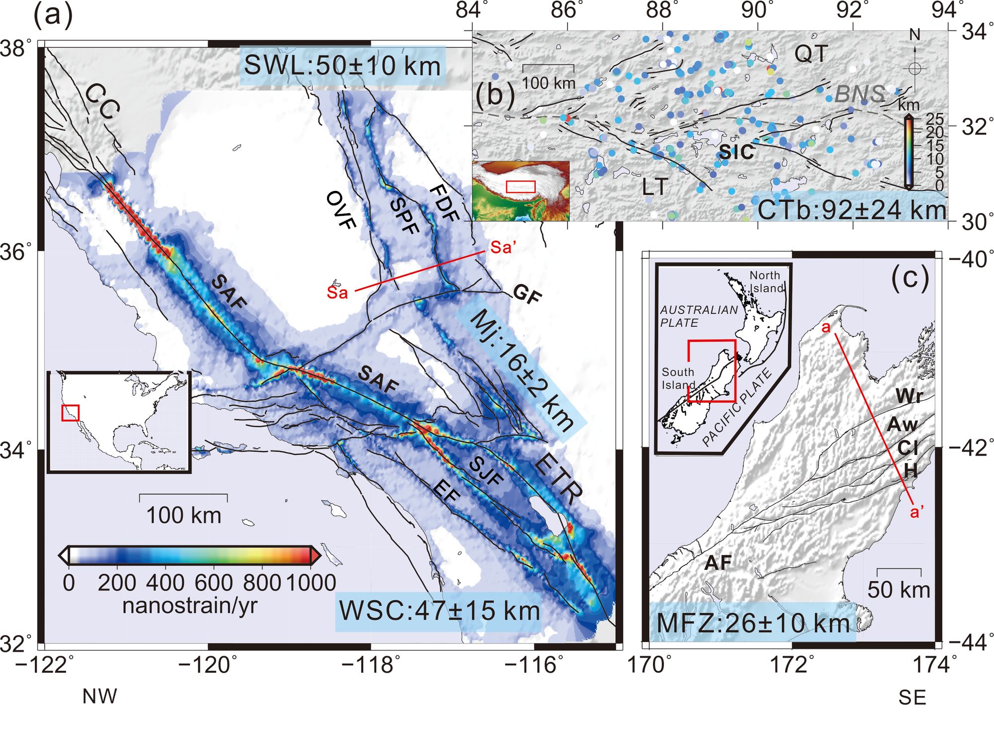
Figure 1. Simplified tectonic maps showing evenly spaced faults (thin black lines) in California (a), central Tibet (b), and New Zealand (c). Numbers in cyan-faced boxes indicate fault spacing in corresponding areas.
Why fault spacing varies with different tectonic settings is not well understood. We derived a scaling relationship that links the fault spacing in continental strike-slip shear zones to other parameters such as fault depth, frictional strength, lower crustal viscosity, etc. The work is published in Journal Earth and Planetary Science Letters.
 Author links open overlay panelHaibinYangaLouis N.MoresiabMarkQuigleya
New scaling model
To determine controls on the spatial distribution of fault traces, they first assume a structurally and rheologically homogeneous material for the model in order to seek a more fundamental understanding of lithospheric scale controls on fault spacing. They first make a force balance analysis for the upper brittle layer with a prescribed basal shear stress to obtain the first-order governing equation for fault spacing. Then, a more self-consistent model describing shear stress at the bottom of a brittle layer(or top of the viscous layer) is derived as a solution to a Laplace equation. They find the fault spacing ($\textit{L}$) can be described by
$L = \frac{C \delta \mu \rho g H^2}{\dot{\varepsilon} \eta}$
where $C$ is a constant number related to the spacial stress decay from a fault, $\delta \mu$ the strength contrast between a fault and surrounding rocks, $\rho$ rock density, $g$ gravitational acceleration, $H$ brittle fault cutting depth, $\dot{\varepsilon}$ strain rate of a fault, $\eta$ lower crustal viscosity. This scaling relationship suggests that increasing brittle fault cutting depth, $H$, strength contrast between faults and country rocks, $\delta\mu$, or decreasing lower layer viscosity, $\eta$, and background strain rate, $\dot{\varepsilon}$, can raise fault spacing.
Application
We also use this scaling relationship to infer the potential lower crustal viscosity, $\eta$, using the observed fault spacing,$L$, at the surface and the range of frictional strength contrast, $\delta \mu$, and the cutting depth of a fault, $H$, which is estimated by the seismogenic thickness. We estimate the lower crustal viscosity for the San Andreas Fault system (California), the Marlborough Fault Zone (New Zealand) and central Tibet (see Figure 2).
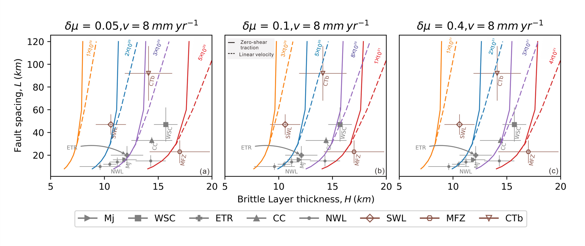
Figure 2. Fault spacing versus brittle fault cutting depth with viscosity contours (unit: Pa∙s) at slip rate of 8 mm yr$^{-1}$ for $\delta\mu$ = 0.05 (a), 0.1 (b) and 0.4 (c).
Co-evolution of fault length, width, and strength
Shallower faults in the early stage of deformation are expected to have closer distances than those in later stages, when they cut deeper. On the other hand, a long (100s km) fault is conventionally thought to evolve by coalescing cracks and smoothing geometrical asperities, which helps to further reduce its strength. Since reducing a fault strength increases the strength contrast between a fault and surrounding rocks, the weakening process also contributes to growing fault spacing.
From the perspective of fault evolution, fault spacing increases over time with increasing H and δμ. The frictional strength is directly linked to the fault plane roughness, which could be inversely related to the accumulated displacement of a fault. The conventional fault growth model suggests the accumulated fault displacements increase with fault lengths (tip-propagation model). The fault growth in length, either through tip propagation or segment linking, tends to increase the stress shadow width, which deactivates smaller faults adjacent to the relatively long fault.
The measured fault spacing should increase with the fault length. In this circumstance, there is a 'safe distance' required for small faults that find themselves adjacent to giant faults, otherwise, the small ones would be eaten by the giant one once they are in the stress shadow of the 'emperor' fault.